Worm Day

I was testing a new version of the Alien Biome made by Bohan, one of our in-house artists. The biome was looking good. I was making sure the new material rendering in UE4 worked as expected. (In case you have not seen it, here is a video showing just that.)


While I roamed around this terrain, I wondered how easily a non-artist like me could extend the scenery. I decided to test what I could achieve in just one day.

I figured out it would be nice to have some massive point of interest. Some sort of giant worm maybe. I loved the Dune treatment by Jodorowsky and Giger. They collaborated mostly about the house Harkonnen. No worms there, but the scale and weight of the concepts was striking. It would be fun to explore a really large formation like the ones they had.

I did not want to create any new textures, materials or props for this. I would be using whatever was already there in this biome. For this reason, I chose to make the giant worm look more like a fossil. Minerals in this planet had taken over every cell of the worm, leaving something that up close looks pretty much like terrain.

The first step was to create a simple model for the worm. I did this using traditional modeling in 3ds max:

This is just a series of primitives arranged in a worm-like fashion, with some worm-tusks sticking out.

The next step was to paint "meta-materials" on top of this. To make it simpler to identify where each meta-material would go, I picked distinct colors to represent each one of them:

In a normal production project, you would have a greater variety of meta-materials. In this case, however, I was really pushing for the minimum amount of work necessary.

Once I had the textured worm, I imported it as meta-mesh in Voxel Studio. I made sure it was huge (3km long) and that it fit nicely the already existing terrain:

I also had to set up some connections between the existing materials and the meta-materials I had painted on top of the model. I chose to use only two meta-materials: one for the tusks and another one for everything else. In this procedural component, each meta-material is subdivided into final materials using artist-created maps. I hoped just two meta-materials was enough to make it interesting.

This part of the setup was quite simple:

After Voxel Studio processed the new mesh and meta-materials, I got to see the worm for the first time:

I was then able to export into Unreal Engine 4 and see how this looked in the final environment. 

I captured this short video so you can have a better idea of the results so far:

While the model and material assignment could use more detail, the sense of scale and weight was already close to what I was looking for. 

I clearly do not have Giger's talent (or Jodorowsky's hallucinogenics supply) so I was curious about how far I could go by myself, and how much the procedural systems we have built could help me. I think it turned out to be OK, considering I only spent around five hours in total creating this feature.

As usual, I look forward to your opinions and comments.

Improved LOD

This is a continuation of an earlier post.

In the past, every Voxel Farm scene could be described by this diagram:

This is a 2D representation of how the entire scene is segmented into multiple chunks. Each chunk may cover a different area (or volume in 3D), but the amount of information in it is roughly the same compared to other chunks, regardless of their size.

Thanks to this trick we can use bigger chunks to cover more distant sections of the scene. Since the chunk is far away, it will appear smaller on screen so we can get away with a much lower information density for it.

Until recently the only criteria we used to decide chunk sizes was how distant the chunk was from the viewer, which is the red dot in the image. For some voxel content types like terrain, we could afford to quickly increase the chunk size along distance to the viewer. The resulting lower density terrain would still look alright.

Some other types of content, however, required more detail. Imagine there is a tower a few kilometers away from the viewer:

The resolution assigned to the chunk containing this tower is simply too low to capture the detail we want for the tower. We could increase resolution to all chunks equally and this would bring the tower into greater detail, but this would be very expensive because many chunks containing just terrain would have their density bumped up as well.

The solution is simple. Imagine that while we build this world, we can compute an error metric for each larger chunk based on the eight (or four in 2D) children chunks it contains. For terrain-only chunks this error would always be zero. For the chunks containing the artist-built tower, this error could be just a counter of how many voxels in the larger chunk failed to capture the detail in the voxels from the smaller children chunks.

Starting from the distance-based configuration we can do another round of chunk refinement. Each chunk having an error that we consider too high will be subdivided. We can keep doing this until the errors are below the allowed threshold and the overall scene complexity remains within bounds.

This gives us a new scene setup:

As result of the additional subdivision, we now use higher density chunks to represent the tower. Since we know how distant these are, we could even pick a chunk size that shows no degradation at all as all errors become sub-pixel on screen.

The following video shows more about this technique:

In the last part of the video, you can see how the terrain LOD changes while the tower remains crisp all the time. If you would also like to minimize terrain LOD changes, this technique can give you that as well:

Just like we can focus the scene more on fine architectural details, we can "unfocus" sections we know will be fine with lower information density.

There is still one issue this technique does not address. When we are bumping up the level of detail of a distant castle, this may also bring a lot of information we do not necessarily want, like walls and spaces that may be inside the castle.

We found a very elegant way to deal with this. This is what enabled the very complex Landmark builds from the earlier post to display in high detail and still run at interactive rates. How we did it will be the topic of the final post on the LOD series. 

Slaying the LOD monster

LOD, or Levels of Detail, is a technique for managing very large and dense scenes like we have today in open world games. The general idea is you can have multiple copies of the same content at different resolutions. Then you switch which copy to use depending on how much detail is necessary for the scene.

LOD switches can be implemented as plain swaps, morphing between states as shown in this earlier post, or even as completely adaptive mesh representations, as shown here.

Sometimes we get fixated on LOD swaps and we drift away devising tricks to make them harder to see. I feel this is not the right angle to look at this problem. While LOD swapping techniques are very important, and progressive swaps are much nicer, etc., the real goal is to have as much detail as possible in the first place. If you find yourself masquerading LOD swaps, it is probably because your scenes still include levels of detail that are too coarse.

How much detail do you need? Just enough to make LOD transitions close to being sub-pixel. Once LOD swaps are sub-pixel, it does not matter what swapping technique you use. It also means your rendering of the content is as detailed as the screen resolution will allow.

This sounds like a Holy Grail, is it feasible with the current hardware generation? We believe it is. Take a look at the following video:



As you can see in the video, buildings preserve their detail, even when viewed from afar. LOD changes, while they do happen, are virtually impossible to detect. All this while keeping interactive frame-rates.

It turns out the same techniques that prevent buildings in the distance from looking like melted crayons also give you smooth LOD transitions. I will be covering how all this works in my next post.

Introducing Farm Cloud

We have included a preview of our collaborative edition system in the latest Voxel Farm 3 release.

The following short video shows what takes to setup and share a project from scratch:

We are still working on this system, but hopefully you get the idea. Our focus is to make the setup as simple as possible so people can start collaborating without significant effort.

This is also intended for more than collaboration and source control. This same layer of distributed persistence can be used by any application to store and sync the changes their users make.

This is a very active area of development for us. I will be posting more about this in the future, meanwhile as always I look forward to the questions you may have about this system.

Pyramid Scene in UE4

Here you can see a video of the Pyramid scene from the previous post:



There are many improvements in this new engine version. Aside the new features like textured voxels and procedural materials, we invested a big deal of time in the quality of the experience. There is still some pop-in, which is coming from a little bug in the meta-material layer. Aside from that the LOD changes are pretty stable and unnoticeable for the most part. The use of UV-mapped voxels also helps minimize the pop-in.

Another old problem area was the replanting of procedural flora (and other objects) every time there was an edit. The new instancing system provides a stable representation that is able to transfer the flora planting into the new geometry. Only edits that really affect the planted instances result in a visual change.

The destruction and building shown here is controlled by blueprints inside UE4. You could easily switch the bombs by a pickax or by rockets.

System Integration

Here is a scene that combines all the recent developments in Voxel Farm:

This integration is subtle. There are no giant turtle mountains here, but the same system we used for the giant turtle is applied here to produce the natural rock pillars that are connected by the bridges, also the platform where the pyramid rests:

These natural structures are defined by a low resolution mesh that captures the basic shape. This is expanded in realtime into detailed features like rocks, sand and dirt using procedural materials that we call Meta-materials.

The large terrain around the pillars and the pyramid's base is using Voxel Farm's standard procedural terrain.

This scene also uses UV-mapped voxels. This is a different method to apply textures to voxels. It allows much finer control. The entire pyramid is using them:

There is also the new instancing system, which is responsible for all the trees plants and rocks you see scattered around. You cannot see this in just screenshots, but this new system is able to preserve existing instances even in the event of user edits and destruction. This avoid the visible "replanting" of vegetation and rocks around edits.

And all this is running in Unreal Engine 4. I would say the UE4 integration is the last of the systems than went into taking these shots.

Intelligent Terrain Synthesis

Don't you hate it when your favorite TV series puts out an episode that is just clips of stuff that happened in earlier episodes? This post has some of that but hopefully will provide you with a better idea of how we see Procedural Generation in the near future.

This video shows the new procedural terrain system to be released in Voxel Farm 3:



In case you want to find out more about what is happening under the hood, these previous posts may help:

Geometry is Destiny Part I and Part II
Introducing Pollock
Terrain Synthesis

The idea is simple. Instead of asking an artist to labor over a hundred of different assets, either by hand or by using complex generation tools like World Machine, we now have a synthetic entity that can do some of that work through a mix of AI and simulation. You do not have to be an expert or initiated at all in the arts of procedural generation to get a satisfactory outcome.

Why are AI and simulation important? After working for a while in procedural generation, it became clear to me there was no workaround to the entropy problem. This I believe can be stated like this: Viewers of procedurally generated content will perceive only the "seed" information, not the "expanded" data. Yes, you may have a noise function that can output terabytes of data, but all this data will be compressed by the human physique to the few bytes that take to express the noise function itself. I posted more in detail about this problem here:

Uncanny Valley of Procedural Generation
Procedural Information
Evolution of Procedural

This does not mean all procedural generation is bad. It means it must produce information in order to be good. Good Procedural Generation is closer to simulation, automation and AI. You cannot have information without work being done, and if work is to be done better leave it to the machine.

The video at the top shows our first attempt at having AI that can do procedural generation, stay tuned because more is coming.

Geometry is Destiny Part 2

This is a continuation of an earlier post. That post ended in a literal, virtual cliffhanger. We generated continent shapes and we used tectonic plate simulation to compute where mountain ranges would appear.

The remaining step was to assign biomes. We wanted biome placement to be believable so we did a bit of research on what biomes are where and why they appear.

Scientists have distilled this to a very convenient set of rules, which are captured by the following chart:

I stole this particular image from Mugan's Biology Page, but you will find it pretty much everywhere occurrence of biomes on Earth is discussed. This is a classification made by Robert Whittaker based on annual precipitation and average temperate. His study suggests temperature and humidity are enough to determine biome occurrence.

This made it simple for us. We only needed to compute two parameters across the continent: temperature and humidity.

Let's start with the easiest, which is temperature. We figured out some of this would have to be user input. as we did not know the latitude for the continent we would not be able to determine how cold or hot it was. Instead of asking how much sun the landmass was getting (which is what latitude means in this case), we chose to ask temperature values for each corner of the map:

To get the temperature for any position within the map we just do a linear interpolation from these four corner values.

Temperature also changes with elevation. This ranges from -6 to -10 degrees Celcius for each extra kilometer in altitude. We had a rough elevation map from the tectonic plate simulation, with this additional piece we are able to compute a fairly good temperature value for any point on the map. This is the horizontal axis of the Whittaker chart.

The vertical axis is rainfall or humidity percentage as other biome charts have it. This one is trickier. In real life, water evaporates from large water masses like the sea into clouds. Air rises when it meets higher elevation. There it cools down losing some of its ability to hold water. The water excess becomes rainfall.

We chose to simulate exactly that process. We knew the continent would be surrounded by ocean water. This would be the main source of water. The next step would be to determine wind direction. Continents are exposed to different wind systems depending on where they are on the planet. Global wind simulation was out of scope for us, so we chose again to ask the user:

The input is quite simple, just a wind direction for each map of the corner. With this, we would be able to produce a wind vector field for the entire map.

If you remember the previous post, a key aspect of this simulation framework was the use of a mesh instead of a regular 2D grid:

This came handy for simulating water transfer. Each node is seeded with an initial amount of water. Nodes over the ocean would get 100% and nodes over the landmass would get zero.

Then we perform multiple simulation steps. Each step looks at each pair of connected nodes and figures out how much water moved from one node to the next and how much was lost as precipitation.

Assume two connected nodes, A and B. The dot product between the wind vector at A, and the vector that goes from A to B will tell us how able the wind is to carry water from A to B. Then based on the water already contained in A and B, and the temperature changes, we can compute how much water moved and how much rainfall there is.

After sufficient simulation steps to cover the node graph, the following pattern emerges:

Here the wind comes from the south. The grayscale shows humidity. The red areas show where the mountains are. As you can see most of the moisture carried by the wind precipitates right after entering the continent, leaving most of the land behind very dry.

If we switch wind direction to the north, a very different pattern emerges:

Once both temperature and humidity are known, assigning biomes is trivial. You can think of the Whittaker chart as a 2D matrix. Humidity determines which row you would use and temperature the column:

This could be generalized to other biome types by providing a different matrix, but I have not paid too much attention to other-worldly biome systems. I have not found any good examples of biome attribution beyond temperature and humidity.

Once you know the biome for each node in the mesh, obtaining a 2D map is a matter of drawing each triangle in the mesh to a bitmap. We had a software rasterizer for occlusion culling that came pretty handy here.

I leave you with a few examples of what happens when you play with wind directions and base temperatures:

A speed build

OK, I am no Shattari or Ginsan (or insert your favorite master-builder here) but I gave it a run at the latest UI in Voxel Studio 3 just to see if it felt right. You can see a live capture here:



This build used lots of UV-mapped meshes. Well, it uses two or three different meshes many times over. This feels closer to building with props with the difference they are fully voxelized so you can copy-paste, deform, and continue to mess with them. When they intersect each other they behave like any other voxel content, you do not get hidden faces, you get only the surface. The mesh is gone after you voxelize it, which is a good thing otherwise this build would have dozens of thousands of individual props.

This was around two hours of work. I had little idea of what I was doing. You can tell I did not prepare well and I got a bit anxious to finish the bottom part so I could go to bed. However, I did like how the tools are arranged in the new UI.

I can hardly wait until this new generation of tools reaches the very talented (and patient) builders out there.

Introducing Pollock

Pollock is the code-name for our new terrain generation system. Why Pollock? This system went rogue for a couple of days and started producing things that did not look like terrain and more like Jackson Pollock paintings:

It seems mad randomness at first, just like Pollock, but there is a lot of order in this chaos (and also what appeared to be a buffer overrun error somewhere in the code.)

Here are some images of the system when it behaves as expected:

The colors you see in these renders are not the final landscape colors. Each color identifies a different layer of more detailed material that will go there. These are placeholder materials Pollock is creating for you.

Pollock's main input is photographs, which you provide to suggest the geography of each biome. In case you want to create a full continent, Pollock will ask you some additional basic facts about elevation, temperature and wind direction.

In continents, you will get nice surprises like a desert appearing on one side of a mountain range:

While the other side of the same range is all made of fertile land:

This has happened due to all the moisture coming from the sea precipitating over one side and having only dry air go over the mountains.

It takes around five minutes to set this up from scratch. The system will so some pre-processing for a few minutes (usually less than five) and that's it. In less than 15 minutes you can complete the creation of an entire continent that spans over a dozen different biomes.

We are in the last stages of completion for this system. There are two main features missing: the addition of forests, rocks, etc. and plugging this with the lake generator to get inner lakes. Right now the system only does ocean.

This system will be included in the Voxel Farm 3 release.

A simple creative mechanic

For some people, a pencil is all they need to create something amazing. For others, the blank page can be discouraging. It is not an invitation to create, rather a reminder you may not be a creative person after all.

I see voxels as a creative medium far superior in terms of simplicity to anything that came before. They are closer to working with physical matter, your mind just gets what you need to do. If done right, they can be as simple and intuitive as using a pencil on paper. But again, pencils can be quite daunting.

I keep asking myself if there is a way around this. We all like to feel creative. Is there a framework where technology can help? Dumbing the medium down to large boxes to level the playing field worked for Minecraft, but this giving both Shakespeare and the village idiot a total vocabulary of five words. They may have a good time just do not expect Julius Cesar.

What if you are not asked to create something entirely new after all? Drawing with a pencil is not the only way you can feel good about your creative self. Remember coloring books. They remove all the stress in the creative act, but you still feel you are creating something.

Here is the equivalent of a coloring book using voxels:



If you are a Landmark builder you will know exactly what is going on. The shapes are already there, they are just filled with air. A paint tool converts the user brushstrokes into visible matter by applying the user's material of choice.

I see games in the future exploiting this mechanic. My five-year-old kids had a lot of fun filling up the different shapes I set up for them. A game could make building rich objects and structures very accessible and stress-free by just hinting where things could be built, and leaving enough for the player to discover and decide on their own.

Voxel Farm 3

I'm happy to announce Voxel Farm 3, a new version of our tech, will be available August 2016.

The team has been working hard towards this next major release. There are still a lot of bugs to squash, but pretty much everything included in the release is ready.

The major items in the release are:

• UV-mapped voxels
• Meta-materials and Meta-meshes for large, custom procedural objects
• Improved Unreal Engine 4 Integration
• New instancing system, both voxel and mesh-based
• Intelligent Biome Terrain Synthesis
• Continent and landmass generator

I have covered most of these already in earlier posts. There are some other items under wraps that we have not disclosed yet, mainly because we are not sure if they will make the release.

The new version will bring a new business model. We are dropping the monthly fees and royalty payments. The new model is simple: you purchase for a one-time fee and you get one year of free updates. To make it fair, we have implemented these changes already for the current version. And everyone who has a Voxel Farm 2 license will get an upgrade to version 3 at no additional cost.

Gearing up towards the major release, we have just updated the company's website at: www.voxelfarm.com

There is a new WebGL demo that shows Voxel Farm in action over the web (it is in the Showcase section.) We also added Forums, something our users have been demanding almost since last year's launch. 

Terrain Synthesis

This is just a teaser. We are still working on this, but we got some results that are already good enough to show. It is not about where terrain types appear (that was covered here and here), but how a particular terrain type is generated.

We want to make procedural generation as accessible as possible. Just like a movie director who shows a portfolio of photos and concept art to the CGI team and just says "make it look like this", we wanted the creator to be entirely clueless about how everything works.

This is how it feels to create a new terrain type. You provide a few pictures of it and we take it from there:

This system builds a probabilistic model based on the samples you provide. That is enough to get an idea of the base elevation. On top of that, several natural filters are applied. It turns out we do know a bit more about this landscape. We know how dry it is, what is the average temperature among other things. The only fact we are missing and have to ask about is how old do you think this is. The time scales range from hundreds of millions of years to billions of years. (If you believe your terrain is 6000 years old we cannot accommodate you at the moment.)

You can provide one or more sample pictures. The more pictures you provide, the better, but just one picture is often enough. Ready to see some results? The following terrains were synthesized out of a single photo in every case (do not mind the faux coloring, this is only to indentify the different terrain layers for now):

Providing multiple samples creates some sort of mix, similar to how you find both mother and father features in their kids:

This works with any kind of image. It could be some fancy concept art as seen below:

The natural filters in this case added some realism to the concept, and eroded some of the original hill shape. This could be avoided if you are after a more stylized look. But if you are short on time, and want to prototype different realistic terrains, the ability to quickly sketch something and feed it to the generator is a big help.

Of course you can still look under the hood and tinker with generation frequencies, filter parameters, etc. You can still have terrain models imported from Digital Elevation Models, or from third party software like World Machine. The key here is you do not have to anymore.

I'd be glad to enter into details of how this works if you guys are interested. Just let me know. I still owe the Part 2 of the continent generation. That should come shortly.

Turtle Mountain

If you have ten minutes or so to spare I encourage you to check out this video. The rest of this post will be about how it was done:


The shyamalanian twist here is the guy lives in the back of a giant turtle. (Maybe not so much of a twist since the video title and thumbnail pretty much give it away.)

What you are seeing here is a new Voxel Farm system in action. It gets a very low-resolution mesh as a base and enhances it by adding procedural detail.

I think this is an essential tool for world builders.. Very often procedural generation deprives the creator of control over the large scale features of the terrain. Or, when control is allowed, it comes in the form of 2D maps like heightmaps and masks. There is no way to drive the procedural generation into complicated shapes and topologies like intricate caves, floating islands, wide waterfalls, etc.

We chose a massive turtle mountain to drive the point anything you can imagine can be turned into a detailed terrain. This is how it works:

The first thing you need to do is create a low-resolution mesh for the base of the terrain feature. This project used three of these meshes, one for the turtle's body and shell, another for the terrain protuberance on the top of the shell and one last mesh for a series of caves. Here you can see them:

On their own they were rather simple to produce. The tortoise is a stock model from a third party site. The mountain was done by displacing a mesh using a heightmap that had a fluvial erosion filter applied to it. The cave system mesh is a simple mesh with additional subdivisions and 3D noise applied to it.

These meshes were imported into Voxel Studio (our creative world building tool) and properly positioned relative to each other.

In addition to triangles, the meshes were textured using traditional means. Here you can see the texture that was applied to the turtle body:

Here is how the textured top mountain looks like:

Note how the texture uses single flat colors. Each pixel in the texture represents a terrain type, not an actual color. You can think of these as instructions to be passed down to the procedural generators when the time comes to add detail.

The meshes may appear detailed at this distance, but if you stretched them to cover four kilometers (which is the size of the turtle base in the world), you would see a single triangle span a dozen of meters or more. A single texture pixel would cover several meters. This would make for a very boring and flat environment. Here is where the procedural aspect kicks in.

Each color in a mesh texture represents what we call a "Meta-Material". I have posted about them before: here and here. In general a metamaterial is a set of rules that define how a coarse section of space can be refined. In this particular implementation for our engine, this is achieved by supplying two different pieces of information:

1. A displacement map
2. A sub-material map 

This is a very simple and effective way to refine space. The displacement map is used to change the geometry and add volumetric detail to an otherwise flat surface. The submaterial map registers closely to the displacement map so the artist can make sure materials appear at the right points in the displaced geometry. Once again the submaterial map does not contain final colors. Each pixel in this map represents a final voxel material that would be applied there.

Here you can see the displacement and submaterial map used for one of the metamaterials in the scene:

One particularly nice aspect of the system is that displacement properly follows the base mesh surface. It is possible to have nice looking cliffs and even apply displacement to bottom facing surfaces like the ceiling of a cave. For mesh-only displacement this is not usually difficult, but doing so in voxel space (so you can dig and destroy) can be quite complex. I'm happy to see we can have voxel cliffs that look right:

Metamaterials, beside displacement and submaterial maps, can be provided with "planting rules". This allows bringing in additional procedural detail in the form of larger instanced content. These can be voxel instances like the large rocks and boulders seen in the video or, they can be passed as instances to the rendering side so a mesh is displayed in that position. The trees in the video are an example of the later.

The previous image shows a mesh instance (a tree) at the left and a voxel instance (a boulder) at the right. Plants, grass, and small rocks are also instanced, but they are planted on top of materials, not meta-materials. One thing I did not mention before is this demo uses Unreal Engine 4. That is another key piece of tech that is coming along very nicely.

Already confused by these many levels of indirection? It is alright, once you start working with these features they begin to make perfect sense. More to that, it becomes apparent this is the only way you can get from a very coarse world definition into something detailed as seen in the video.

I hope you enjoyed this and that it gets your imagination started.

Applying textures to voxels

When I look back at the evolution of polygon-based content, I see three distinct ages. There was a time where we could only draw lines or basic colored triangles:

One or two decades later, when memory allowed it, we managed to add detail by applying 2D images along triangle surfaces:

This was much better, but still quite deficient. What is typical of this brief age is that textures were not closely fitted to meshes. This was a complex problem. Textures are 2D objects, while meshes live in 3D. Somehow the 3D space of the mesh had to be mapped into the 2D space of the texture. There was no simple, single analytical solution to this problem, so mapping had to be approximated to a preset number of cases: planar, cylindrical, spherical, etc.

With enough time, memory constraints relaxed again. This allowed us to write the 3D to 2D mapping as a set of additional coordinates for the mesh. This brought us into the last age: UV-mapped meshes. It is called UV because it is an additional set of 2D coordinates. Just like we have XYZ for the 3D coordinates in space, we use UV for coordinates in the texture space. This is how Lara Croft got her face.

We currently live in this age of polygon graphics. Enhancements like normal maps, or other maps used for physically based rendering, are extensions of this base principle. Even advanced techniques like virtual texturing or Megatextures still rely on this.

You may be wondering why is this relevant to voxel content. I believe voxel content is no different than polygon content when it comes to memory restrictions, hence it should go through similar stages as restrictions relax.

The first question is whether it is necessary to texture voxels at all. Without texturing, each voxel needs to store color and other surface properties individually. Is this feasible?

We can look again to the polygon world for an answer. The equivalent question for polygon content would be, can we have all the detail we need from just geometry, can we go Reyes-style and rely on microgeometry? For some highly stylized games maybe, but if you want richer realistic environments this is out of the question. In the polygon realm this also touches the question about use of unique texturing and megatextures, like in idTech5 and the game Rage. This is a more efficient approach on having a unique color per scene element, but still was not efficient enough to compete with traditional texturing. The main reason is that storing unique colors for entire scenes was simply too much. It led to huge game sizes while the perceived resolution remained low. Traditional texturing on the other hand allows to reuse the same texture pixel many times over the scene. This redundancy decreases the required information by an order of magnitude at often no perceivable cost.

Unique geometry and surface properties per voxel are no different than megatextures. They are slightly worse as the geometry is also unique, and polygons are able to compress surfaces much more efficiently than voxels. With that in mind, I think memory and size constrains are still too high for untextured voxels to be competitive. So there you have the first voxel content age, where you still see large primitives and flat colors, and size constraints won't allow them to become subpixel:

(Image donated by Doug Binks @dougbinks from his voxel engine)

The second age is basic texturing. Here we enhance the surface detail by applying one ore more textures. The mapping approach of choice is tri-planar mapping. This is how Voxel Farm has worked until now. This is sufficient for natural environments, but still not there for architectural builds. You can get fairly good looking results, but requires attention to detail and often additional geometry:

In this scene (from Landmark, using Voxel Farm) the pattern in the floor tiles is made out of voxels. The same applies to table surfaces. These are quite intricate and require significant data overhead compared to a texture you could just fit to each table top for instance, as you would do for a normal game asset.

We saw it was time for voxels to enter the third age. We wanted voxel content that benefited from carefully created and applied textures, but also from the typical advantages you get from voxels: five-year-olds can edit them and they allow realistic realtime destruction.

The thing about voxels is, they are just a description of a volume of space. We tend to think about them as a place to store a color, but this is a narrow conception. We saw that it was possible to encode UV coordinates in voxels as well.

What came next is not for the faint of heart. The levels of trickery and hackery required to get this working into a production ready pipeline were serious. We had to write voxelization routines that captured the UV data with no ambiguities. We had to make sure our dual contouring methods could output the UV data back into triangle form. The realtime compression had to be now aware of the UV space, and remain fast enough for realtime use. And last but not least we knew voxel content would be edited and modified in many sorts of cruel ways. We had to understand how the UV data would survive (or not) all these transformations.

After more than a year working on this, we are pleased to announce this feature will make it into Voxel Farm's next major release. Depending on the questions I get here, I may get more into detail about how all this works. Meanwhile enjoy a first dev video of how the feature works:

Geometry is Destiny

In the previous post, I introduced our new land mass generation system. Let's take a look at how it works.

For such a large thing like a continent, I knew we would need some kind of global generation method. Global methods involve more than just the point of space you are generating. The properties for a given point are influenced by points potentially very far away. Global methods, like simulations, may require you to perform multiple iterations over the entire dataset. I favor global methods for anything larger than a coffee stain in your procedural table cloth. The reason is they can produce information whereas local methods cannot: information is limited to the seeds used in the local functions.

The problem in using a global simulation is speed. Picking the right evaluation structure is paramount. I wanted to produce maps of approximately 2000x2000 pixels, where each pixel would cover around 2 km. I wanted this process to run in less than five seconds for a single CPU thread. Running the generation algorithm over pixels would not get me there.

The alternative to simulating on a discrete grid (pixels) is to use a graph of interconnected points. A good approach here is to scatter points over the map, compute the Voronoi cells for them, and use the cells and their dual triangulation as the scaffolding for the simulation.

I had tried this in the past with fairly good results, but there was something about it that did not sit well with me. In order to have pleasant results, the Voronoi cells must be relaxed so they become similarly shaped and the dual triangulation is made of regular triangles.

If the goal was to produce a fairly uneven but still regular triangle mesh, why not just start there and avoid the expensive Voronoi generaion phase? We would still have implicit Voronoi cells because they are dual to the mesh.

We started from the most regular mesh possible, an evenly tessellated plane. While doing so we made sure all diagonal edges would not go in the same direction by making their orientation flip randomly:

Getting the organic feel of the Voronoi driven meshes from here was simple. Each triangle is assigned a weight and all vertices are pulled or pushed into triangles depending on these weights. After repeating the process a few times you get something that looks like this:

This is already very close to what you would get from the relaxed Voronoi phase. The rest of the generation process operates over the vertices in this mesh and transfers information from one point to another using the edges connecting vertices.

With the simulation scafolding ready, the first actual step into creating the land mass is to define its boundaries. The system allows a user to input a shape, in case you were looking for that heart-shaped continent, but if no shape is provided a simple multiresolution fractal is used. This is a fairly simple stage, where vertices are classified as "in" or "out". The result is the continent shoreline:

Once we have this, we can compute a very important bit of information that will be used over and over later during the generation: the distance to shoreline. This is fairly quick to to compute thanks to the fact we operate in mesh space. For those triangle edges that cross the shoreline we set the distance to zero, for edges connected into these the distance is +1 and so on. It is trivial to produce a signed distance if you add for edges in mainland and subtract for edges in the ocean.

It is time to add some mountain ranges. A naive approach would be to use distance to shore to raise the ground, but this would be very unrealistic. If you look at some of the most spectacular mountain ranges on Earth, they happen pretty close to coast lines. What is going on there?

It is the interaction of plate tectonics what has produced most of the mountain ranges that have captured our imagination. This process is called orogeny, and there are basically two flavors of it, accounting for most mountains on Earth. The first is when two plates collide and raise the ground. This is what gave us the Himalayas. The second is when the oceanic crust (which is a thinner New-York-pizza-style crust) sinks below the thicker continental crust. This raises the continental crust producing mountains like the Rockies and the Andes. The two processes are necessary if you look for a desirable distribution of mountains in your synthetic world.

Since we already have the shape of the continental land, it is safe to assume this is part of a plate that originated some time before. More-so, we can assume we are looking at more than one continental plate. This is what you see when you look at northern India, even if it is all a single land mass, three plates meet at this point: the Arabian, Indian and Eurasian plates.

Picking points fairly inland, we can create fault lines going from these points into the map edge. Again this works in mesh space, so it is fairly quick and the results have the rugged nature we initially imprinted into the mesh:

Contrary to what you may think, this is not a pathfinding algorithm. This is your good-old midpoint displacement in action. We start with a single segment spanning from the fault source to the edge of the map. This segment, and each subsequent segment, is refined by adding a point in the middle. This point is shifted along a vector perpendicular to the segment by a random amount. It is fairly quick to know which triangles are crossed by the segments so the fault can be incorporated into the simulation mesh.

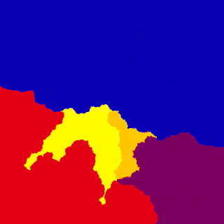
In this particular case the operation has created three main plates, but we are still missing the oceanic plates. These occur a bit randomly, as not every shoreline corresponds to an oceanic plate. We simulated their occurrence by doing vertex flood fills on selective corners of the map. Here you can see the final set of plates for the continent:

The mere existence of plates is not enough to create mountain ranges. They have to move and collide. To each plate we assign a movement vector. This encodes not only the direction, but also the speed at which the plate is moving:

Based on these vectors we can compute the pressure on each vertex and decide how much it should be raised or lowered, resulting in the base elevation map for the continent:

All the mountains happened to occur in the South side of the continent. You can see why this was determined by the blue plate drifting away from the mainland, otherwise we would have had a very different outcome. This will be an interesting place anyway. While the gray-scale image does not show it, the ground where the blue plate begins sinks considerably, creating a massive continent-wide ravine.

Getting the continent shape and mountain ranges is only half the story. Next comes how temperature, humidity and finally biomes are computed. Stay close for part two!